Table of Contents
Simple MAGNETIC simulation in FEMM - step-by-step tutorial
This page shows a step-by-step tutorial of a very simple magnetic simulation.
Other tutorials:
| Helpful page? Support Encyclopedia Magnetica. All we need is $0.25 per month? Come on… |
Step 1 - solver
Open FEMM and start new problem, menu > File > New .
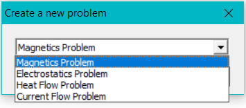
Select Magnetics problem from the pop-up window (Fig. 1).
Step 2 - problem
Set problem and unit conditions (Fig. 2) from menu > Problem, and choose: Planar, Millimeters, Frequency = 50 Hz, Depth = 10 mm (the rest leave with default values). If you use the settings as shown in Fig. 2 then you can compare with this tutorial if the calculation is correct.
 Fig. 2. Set problem and unit conditions
Step 3 - points
Click on “Nodes” button (Operate on nodes) (Fig. 3-1).
 Fig. 3-1. “Nodes” button selected
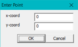
Press TAB (on keyboard) to manually input a node (point) with coordinates (Fig. 3-2). Enter the following points:
- point
x = 0, y = 0 - point
x = 1, y = 0 - point
x = -2, y = -2 - point
x = -2, y = 2 - point
x = 2, y = -2 - point
x = 2, y = 2 - point
x = -3, y = -3 - point
x = -3, y = 3 - point
x = 3, y = -3 - point
x = 3, y = 3
 Fig. 3-2. Entering point with coordinates (0,0)
Click on the Zoom extents button (Fig. 3-3), which is the third one (white rectangle with a magnifying glass). (If not sure - hover a mouse over the buttons and see their description in the bottom left of the FEMM window.)
Then click on the Zoom out button once (magnifying glass with a minus).
 Fig. 3-3. Zooming buttons, from left: Zoom in, Zoom out, Zoom extents, Zoom to window
If everything is done correctly, the window should look like in Fig. 3-4.
Step 4 - lines
Select the “Line” button (Operate on segments, see also Fig. 3-1). Draw a line between two nodes by clicking on the first point, then on the second point. Draw all lines so that a “frame” is created as in Fig. 4-1.
 Fig. 4-1. Frame is created with straight lines
Step 5 - arcs
Select the “Arc” button (Operate on arc segments) (see also Fig. 3-1).
The arcs are always drawn in anti-clockwise direction. So to draw a bottom arc as shown in Fig. 5-1 the points have to be clicked in the sequence “1” then “2”. To draw the top arc click “2” then “1”.
 Fig. 5-1. Bottom arc from 1 to 2, top arc from 2 to 1
Step 6 - copy
The inner circle consists of nodes and arcs. These can be copied separately, but also can be copied as one object, which can be done by executing the following sequence (Fig. 6-1):
- 1. Select Operate on group of objects button
- 2. Click on Select a group of entities using the mouse (the button will not stay depressed)
- 3. Draw a rectangle around the object to be copied
- 4. Click on Copy selected objects and enter
Horizontal shift = 4
If all was executed correctly the geometry should look like in Fig. 6-2.
Step 7 - save
Save the file: menu > File > Save
Step 8 - circuits
To set the current in conductors or circuits go to: menu > Properties > Circuits
Several currents can be specified and used for separate windings or conductors. A new circuit can be added by Add Property (Fig. 8-2), and filling the value of current in the Circuit Property pop-up window.
The phase of the current is specified by using complex notation. For example, the value of 0.7071+I*0.7071, means that there is 0.7071 of the real component (0 deg. phase) and +I*0.7071 means the imaginary component (90 deg. phase), so this combination represents a peak current of 1.000 A at 45 deg. phase.
FEMM only solves with current as the input variable. It is not possible to set voltage. If the voltage needs to be used then some iterative calculations are required (especially with non-linear materials). External calculations are required. See an example here: https://www.femm.info/wiki/MyTransformer
 Fig. 8-2. Add current / circuit
Step 9 - material library
FEMM contains a library / database of materials, which can be used in the model, Fig. 9-1.
 Fig. 9-1. Accessing Materials Library
The library window has two parts. On the left (“database” in Fig. 9-2), there are all the available materials as provided by FEMM. New materials can be added to it if needed.
The part on the right is for all the materials which will be accessible within the given model. Simply use the mouse to drag-and-drop method to drag the given material from the left to the right sub-window.
 Fig. 9-2. Database (left) and model (right), drag-and-drop
Step 10 - boundary
FEM equations require boundary conditions to be solved. They act as a reference point. Many different conditions can be specified, but for a simple magnetics simulation it is typically most useful to use the built-in “open boundary” feature. This boundary simulates an infinitely large volume (hence “open”), even though it can be positioned quite close to the simulated objects.
This “open boundary” method (Fig. 10-1) should be done only after all other geometry was created, because it can automatically set the right size of the boundary, suitably larger than the rest of the model. If this is the case then nothing needs to be changed in the pop-up window, and all the default values can be accepted with “OK”.
 Fig. 10-1. Create open boundary automatically
After accepting there will be many circles created automatically, Fig. 10-2. There will be some block names appearing in the circles (as shown by the red arrows). These should be ignored, because they are needed for correct operation of the boundary.
 Fig. 10-2. Open boundary created
Step 11 - block labels, materials, currents
Every part in the model must have a material data assigned to it, so FEMM know how to solve it. Each area completely surrounded by blue lines or arcs represents a “block”, and each such block has to have the material specified for it. This is done by using the green icon Operate on block labels, Fig. 11-1.
After selecting the option click somewhere (anywhere) inside of each block, as shown in Fig. 11-1. A green point called <none> will appear with each click. To remove it, just right-click on it (to select it, changes colour to red) and press Delete (on keyboard).
Then each green point has to be configured. Right-click on a given point and press Space (on keyboard). Alternatively, after selecting (it turns to red) use: menu > Operation > Open selected. A pop-up window will appear, Fig. 11-2.
In the window, use the drop down list to select material type or “Block type”. For example, Air is chosen for the point in Fig. 11-2. If the material is passive (no current flowing, not a magnet), then nothing more needs to be configured. Press OK to accept.
The drop down list will also contain the u1, u2, u3… materials for the open boundary. These should be ignored.
Notes:
- You can select more than one point, and all the selected points can be configured simultaneously.
- Unchecking the box allows setting manual mesh size (described below).
- The “In group” variable can be used to group some objects. All objects have by definition group = 0. But this can be set to other value so that several objects can be a part of the same group. This is useful for editing (move, copy, rotate) or results analysis (select all objects in the group easily).
 Fig. 11-2. Configure block labels
If the given block has some imposed current flowing through then it is also set in the same window. Fig. 11-3 and Fig. 11-4 show how to set current in the circular wires. FEMM uses the approach of “positive turns” and “negative turns” for the same current. So just one current needs to be defined and the values have to be assigned as shown in the figures.
There is no need to draw each individual wire. It is sufficient to draw the whole rectangular cross-section shape of the coil and assign a number of turns the the whole area (such that N > 1).
The frame core is configured as “Pure iron” in the final model, Fig. 11-4.
Step 12 - mesh
Before meshing - save the file! A very large mesh can sometimes cause problems, so it is a good idea to save before meshing.
For simple models it is sufficient to use the automatic settings of mesh. Just click on the “mesh” button, Fig. 12-1. If all materials were assigned to all blocks then the pop-up message states just the number of nodes of the mesh, meaning that all is correct.
If some block label was left undefined then this message will say something like:
| Created mesh with 12239 nodes. Grey mesh lines denote regions that have no block label. |
It is necessary to define ALL block labels.
 Fig. 12-1. Mesh (automatically generated)
Step 13 - analyse / solve
Analysis is executed by clicking the “cranked cog” icon (red arrow in Fig. 13-1). A pop-up window appears which shows the progress of calculations. Just wait until it finishes. No message is shown if all finishes correctly.
As soon as the small window disappears the results can be viewed by clicking the “glasses” button (black arrow).
For all-linear models the calculation finishes in one step. For non-linear models it takes many iterations. For highly non-linear models (e.g. with deep saturation) or with large very dense mesh, the calculations can take very long time.
If there are errors in the model or material data the solution might not converge. If the computation time is excessive typically there is a problem somewhere in the model (block labels, double labels, wrong boundary, etc.)
Step 14 - results
Clicking the button shown by the black arrow in Fig. 13-1 opens a new window (post-processing), with the results of the simulation loaded. Depending on the configuration of FEMM there could be lines or colours, or no lines and no colours.
The type of data can be selected by using the “lines” or “rainbow” buttons, Fig. 14-1.
These two options can be accessed also through: menu > View > Contour plot and menu > View > Density plot.
 Fig. 14-1. Results window, with field lines, no colour map
Clicking the “rainbow” button shows the small window, which which the type of variable can be selected: Flux density B, Magnetic field intensity H, or Current density J. Limits are scaled automatically between the min. and max. value present in the model, but they can be adjusted manually as needed, Fig. 14-2.
Don't forget to tick the “Show Density Plot” box!
 Fig. 14-2. Choosing Flux density B |T| density plot
Flux density |B| plot with the flux lines disabled is shown in Fig. 14-3.
 Fig. 14-3. Flux density |B| plot
Step 15 - plot data along line
In the solution window, use the “red line” icon (Fig. 15-1) to draw a path of lines or arcs, between any two existing points (left-click of mouse) or between any arbitrary points (right-click of mouse). Once the path is created, various values can be plotter along that line, from the beginning to its end, in the same order as it was drawn.
The path can end at the same point it started.
To plot, press the “graph” icon (Fig. 15-1). A pop-up window will open and the variable to be plotted can be selected, Fig. 15-2. N
Note that there is an option to export/write the data to a file, which can be then used with any spreadsheet software.
 Fig. 15-1. Draw path to plot data
 Fig. 15-2. Select data to plot or export to file
The graph will be opened in a new window. For AC simulations, black curve means the absolute value (total amplitude), blue is the “real” component (0 deg), and green is the “imaginary” component (90 deg).
 Fig. 15-3. New window with plotted data
Step 16 - block integral
Some values can be integrated over the whole blocks. To select a block use the “green square” button, and then click anywhere within a block of interest, Fig. 16-1.
Then click on the “integral” icon.
A pop-up window will appear (Fig. 16-2), and the drop-down list can be used to select the value of interest. After accepting, the value will be evaluated and shown in another pop-up window, Fig. 16-3.
 Fig. 16-2. Select type of integral
 Fig. 16-3. Calculated value of integral
Step 17 - conductor info
The losses in the circuit (energised coil) can be integrated with the block method described above, but much richer information is provided with the “Circuit properties” icon, Fig. 17-1.
If there is more than one current/circuit defined then it can be selected from the drop-down list.
Step 18 - values at any point
Data for any point, anywhere in the model can be easily displayed by enabling the Output Window (Fig. 18-1) and left-clicking anywhere in the model.
If snap-to-grid is enabled then only the grid positions will be available.
 Fig. 18-1. Click anywhere to get values
Step 19 - that's it!
And that's all - now you can run a simple FEMM magnetics simulation!
| Helpful page? Support Encyclopedia Magnetica. All we need is $0.25 per month? Come on… |


